CT Scan Reconstruction with Linear Algebra

A CT scanner measures total X-ray absorption along many ray paths through the body and must recover the density at every pixel. X-ray attenuation follows the Beer-Lambert law:

Discretize the image into pixels and each ray becomes one linear equation. The path length of ray i through pixel j is the coefficient a_ij, the measured absorption for ray i is b_i, and the unknown pixel densities are x_j:

Image reconstruction is solving Ax = b for x.

• Phantom: 4x4, a bright 2x2 "bone" block on a darker "tissue" background
• Projection angles: 4 (0°, 45°, 90°, 135°)
• Noise: 5% Gaussian added to measurements to mimic a real detector

The forward model builds A, computes b = A*x_true + noise, then recovers x_true from b alone.

How the projections build the matrix

Each projection angle contributes a set of rays, and each ray becomes one row of A.

• At 0°, horizontal rays sum the pixels in each row: x₁ + x₂ + x₃ + x₄ = b₁
• At 90°, vertical rays sum each column
• At 45° and 135°, diagonal rays have path length √2 through each pixel rather than 1

The ART update, applied for every ray on every iteration:

with relaxation λ = 0.1, starting from a zero image, for 50 iterations.

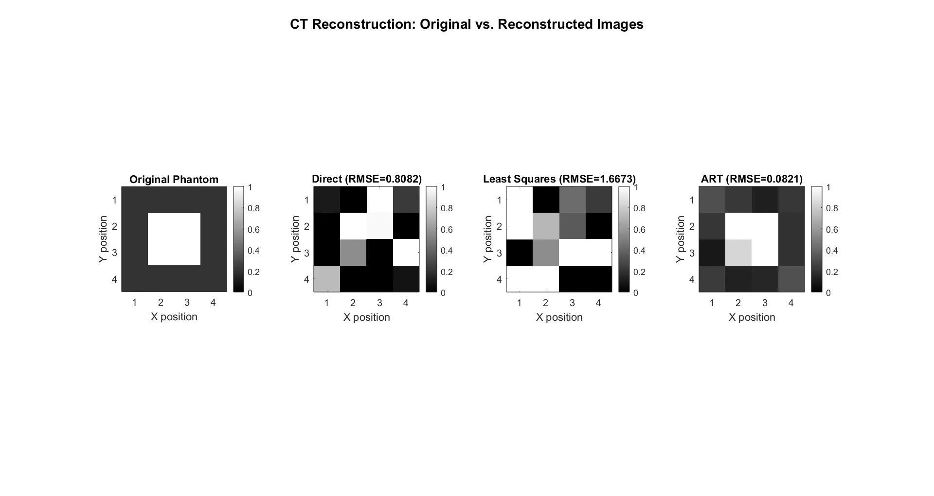
Direct and Least Squares scatter density into the wrong pixels and lose the block entirely. ART is the only method that reproduces a recognizable bright center on a dark background. Least Squares is roughly 20 times worse than ART.

ART starts above 0.4 RMSE, drops below both reference methods within the first handful of iterations, and flattens out near 0.08 by iteration 50.

The four angles produce only 13 rays, but there are 16 unknown pixels. A is 13x16: the system is underdetermined, and its rank is only 12. Consequences per method:

• Least squares solves the normal equations (AᵀA)x = Aᵀb. Because A is rank-deficient, AᵀA is singular (condition number ~10¹⁷). Solving a singular system amplifies the measurement noise instead of averaging it out, which is why least squares gives the worst RMSE rather than the best. The code prints this condition number directly.
• Direct solve (A\b) on an underdetermined system returns a basic solution with at most rank(A) = 12 nonzero entries. Bounded but non-physical, so it captures only part of the image.
• ART does not form AᵀA at all. It projects the current estimate onto each ray constraint in turn, which converges to the minimum-norm solution of the underdetermined system. For this phantom that solution is very close to the true image.

When the system is rank-deficient, the iterative projection method is the robust choice while the normal-equations approach is actively harmful. This is also why real CT scanners, which solve enormous and often ill-conditioned systems, rely on iterative reconstruction rather than direct inversion.

Most of A is empty, because each ray touches only a few pixels. Horizontal and vertical rays contribute 1.0; diagonal rays contribute √2. This is realistic: in a clinical scanner each ray crosses only 10 to 20 of thousands of pixels. With 13 rows of mostly-zero entries, A cannot pin down all 16 unknowns, which is the underdetermined condition driving every result above.

1. The system is underdetermined (13 equations, 16 unknowns). To make least squares behave as theory predicts, A needs to be genuinely overdetermined and well-conditioned: more projection angles (for example 30°, 60°, 120°, 150°) and a full bundle of parallel rays per angle instead of single diagonal rays, so that rank(A) ≥ 16 with margin.
2. The ray model is simplified. Each ray is treated as passing through whole pixels with unit or √2 weights rather than computing the true intersection length through each pixel. A proper forward projector (such as Siddon's algorithm) would make A reflect real scanner geometry.
3. Fixed relaxation and iteration count. ART uses a constant λ = 0.1 and 50 iterations. Adapting the relaxation parameter or adding a residual-based stopping criterion would be more principled.

Systems of linear equations (Ax = b), rank and underdetermined systems, singular matrices and conditioning, sparse matrices, least squares via the normal equations, the Kaczmarz iterative method, matrix-vector operations.

Final project for ENGR 2300 (Linear Algebra for Engineers). The application, the MATLAB implementation, and the analysis are my own.